Table of Contents
To change the format and appearance of selected cell(s), row(s) or column(s) use the option from the menu or from the mouse button popup menu.
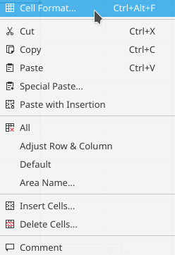
This will bring up the Cell Format dialog box which has several tabbed pages:
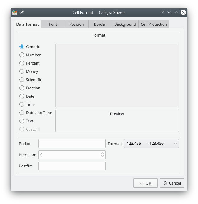
The Data Format page of the Cell Format dialog box lets you control how the values of cells are displayed.
The top part of this page lets you select the format to be used when displaying numeric values, dates or times. A Preview pane allows you to see the effect of the new format.
You can set the same data format for a row or a column by selecting the row or column and calling the Cell Format dialog with the mouse button.
Note
You can increase the precision decimal for any number in Generic,
Number, Percent, Money or
Scientific formats using the Increase
precision icon in the Format toolbar: 
You can decrease the precision decimal for any number in Generic,
Number, Percent, Money or
Scientific formats using the Decrease precision icon
in the Format toolbar: 
- Generic
This is the default format and Calligra Sheets autodetects the actual data type depending on the current cell data. By default, Calligra Sheets right justifies numbers, dates and times within a cell and left justifies anything else.
If the Generic format does not suit you, you can change to a specific format among the choices below.
- Number
The number notation uses the notation you globally choose in System Settings in → → . Numbers are right justified by default.
- Percent
When you have a number in the current cell and you switch the cell format from Generic to Percent, the current cell number will be multiplied by 100.
For example if you enter 2 and set the cell format to Percent, the number will then be 200 %. Switching back to Generic cell format will bring it back to 2.
You can also use the Percent icon in the Format Toolbar:

- Money
The Money format converts your number into money notation using the settings globally fixed in System Settings in → → . The currency symbol will be displayed and the precision will be the one set in System Settings.
You can also use the Money Format icon in the Format toolbar to set the cell formatting to look like your current currency:

- Scientific
The Scientific format changes your number using the scientific notation. For example, 0.0012 will be changed to 1.2E-03. Going back using Generic cell format will display 0.0012 again. The Generic cell data format does not keep scientific notation so if you want this notation, you have to specify it using this menu item.
- Fraction
The Fraction format changes your number into a fraction. For example, 0.1 can be changed to 1/8, 2/16, 1/10, etc. You define the type of fraction by choosing it in the field on the right. If the exact fraction is not possible in the fraction mode you choose, the nearest closest match is chosen. For example: when we have 1.5 as number, we choose Fraction and Sixteenths 1/16 the text displayed into cell is "1 8/16" which is an exact fraction. If you have 1.4 as number in your cell and you choose Fraction and Sixteenths 1/16 then the cell will display "1 6/16" which is the nearest closest Sixteenth fraction.
- Date
To enter a date, you should enter it in one of the formats set in System Settings in → → . There are two formats set here: the date format and the short date format.
A random natural number NN will be transformed in the date from 30st December 1899 (which is 0) with the number of days NN added. For example if you have a cell with 100 and you choose Date format, "1900-04-09" will be displayed in the cell which is 100 days after 30st December 1899. This starting date is two days early as it was a bug in Lotus 123 and then it stayed that way in Excel in order to keep compatibility. Few people will need to calculate from 1st January 1900 anyway and adding 9 days to 1st November 2000 for example will give you 10th November 2000 so all normal calculations on dates are correct.
Note
When a cell is in the Date format, you can drag this cell down as you do with numbers and the next cells will also get dates, each date being increased by one day.
- Time
This formats your cell content as a time. To enter a time, you should enter it in the Time format set in System Settings in → → . In the Cell Format dialog box you can set how the time should be displayed by choosing one of the available time format options. The default format is the system format set in System Settings. When the number in the cell does not make sense as a time, Calligra Sheets will display 00:00 in the global format you have in System Settings.
- Date and Time
This formats your cell content as date and time. To enter a date and a time, you should enter it in the Time format set in System Settings in → → . In the Cell Format dialog box you can set how the date and time should be displayed by choosing one of the available date and time format options. The default format is the system format set in System Settings. When the number in the cell does not make sense as a date and time, Calligra Sheets will display 00:00 in the global format you have in System Settings.
- Text
This formats your cell content as text. This can be useful if you want a number treated as text instead as a number, for example for a ZIP code. Setting a number as text format will left justify it. When numbers are formatted as text, they cannot be used in calculations or formulas. It also change the way the cell is justified.
- Custom
Does not work yet. To be enabled in the next release.
The lower part of the Data Format page lets you add a Prefix: such as a $ symbol at the start of each item or a Postfix: such as $HK to the end. You can also control how many digits are displayed after the decimal point for numeric values, whether positive values are displayed with a leading + sign and whether negative values are shown in red.
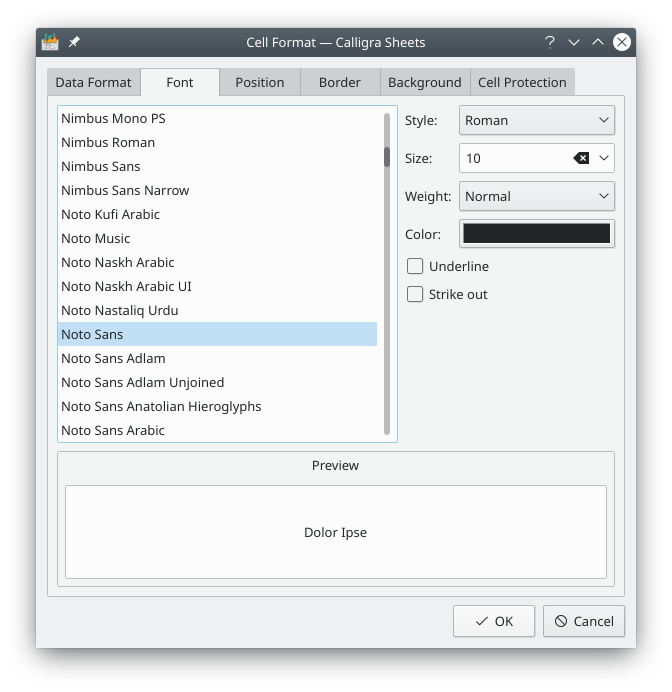
The Font page lets you select the font family, Style:, Size:, Weight: and Color: for the current cell, including some additional options like underlined or striked out text. The lower part of the page gives a Preview of the selected text format.
The default font is set for all cells in the → menu with the currently used style.
- Style:
Choose the style for your font for the currently selected cells. When you select several cells with different styles, the displayed style is set to Varying (No Change) and leaving it that way will keep all your current style settings for each cell. Changing to Roman for example will change all the selected cells style text to Roman.
- Size:
Choose the size for your font for the currently selected cells. When you select several cells with different sizes, the displayed size is set to (no number written) and leaving it that way will keep all your current size settings for each cell. Changing to 14 for example will change all the selected cells font size to 14.
- Weight:
Choose the weight for your font for the currently selected cells. When you select several cells with different font weight, the displayed weight is set to Varying (No Change) and leaving it that way will keep all your current weight settings for each cell. Changing to Bold for example will change all the selected cells font weight to Bold.
- Color:
Choose the color for the currently selected cells' text. Clicking on the color bar will bring you the standard KDE Select Color dialog where you will be able to choose the new color.
- Underline
Underlines the currently selected cells' text if checked. This is not checked per default.
- Strike out
This will strike out the currently selected cells' text if this is checked. This is not checked per default.
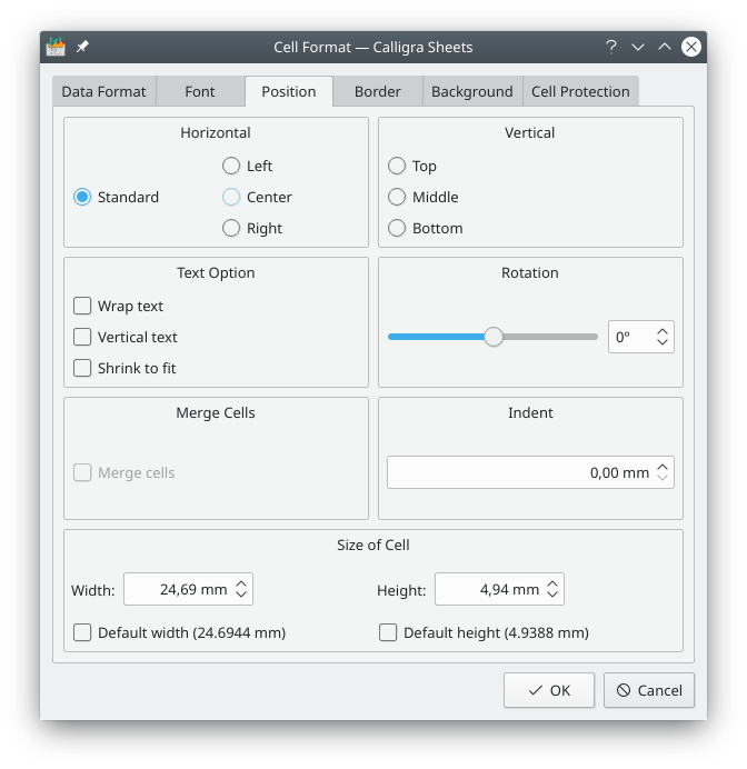
From the Position page you can control the position of text within a cell by making suitable selections in the Horizontal and Vertical areas or by setting the Indent value. You can also choose to have the text appear vertically rather than horizontally, or even at an angle.
- Horizontal
Set the content position horizontally in the cell. Standard is default and is set from the data format you choose. Left means the content will be displayed on the left of the cell. Center means the content will be in the center horizontally in the cell. Right means the content of the cell will be displayed on the right of the cell.
- Vertical
Set the content position vertically in the cell. Top means the content will be displayed on top of the cell. Middle means the content will be in the middle vertically in the cell. Bottom means the content of the cell will be displayed at the bottom of the cell.
- Text Option
This is only available when the rotation is 0°. Wrap text wraps the text so it fits in the previous cell size. If this is not checked, the text will stay on one line.
Vertical text puts your text vertically.
- Rotation
Your text will appear oriented in the angle you set here. Positive values will move it counter-clockwise and negative values will move it clockwise.
- Merge Cells
When checked, this has the same effect as → . You need to have at least two consecutive cells selected. Those consecutive cells are then merged into a bigger one.
When a merged cell is selected and when you uncheck this, then all cells come back to their original size as before the merging. It has the same effect as → .
- Indent
Set the amount of indent that will be used in the cell when you choose the Increase Indent/Decrease Indent actions from the toolbar. These actions are not enabled by default in the toolbar.
- Size of Cell
You set here the size of the cell, either a custom width and height or choose the default width and height.
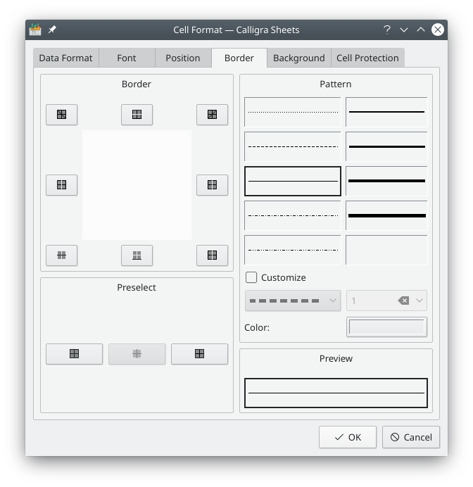
The Border page lets you set the appearance of the cell borders. If you have selected more than one cell you can apply different styles to the borders between the cells and that surrounding the selected area.
First select the pattern and color from the Pattern section of the Border page then apply that to different parts of the border by clicking on the appropriate button in the Border section, or on one of the Preselect buttons. The left hand button in the Preselect section will clear any previously applied border(s). Note that you can also add a diagonal strike-through line to the cell(s).
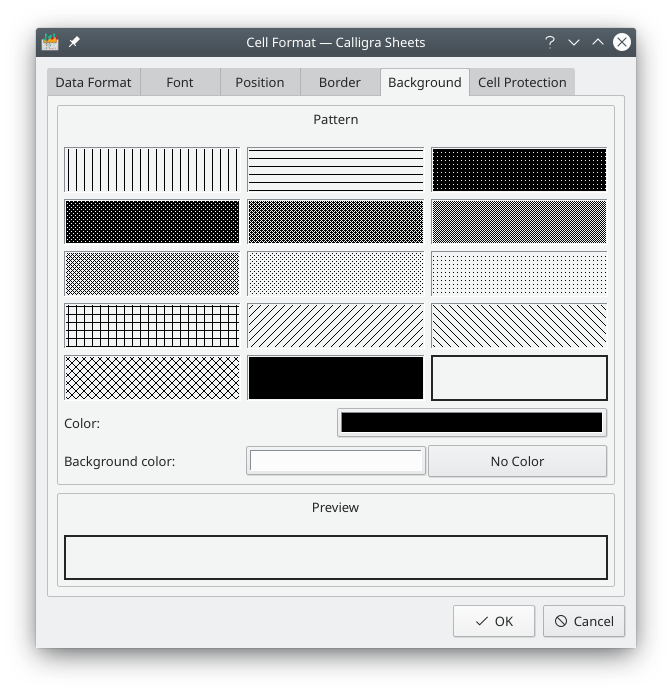
The cell background pattern and color can be selected from the Background page.
Simply choose a desired Pattern, then select the pattern Color and the Background color.
At the bottom of this page you can see a Preview of the configured cell background.
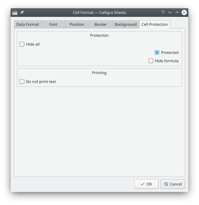
You can change the way the content of a cell is protected in the Cell Protection page.
All cells are protected by default (that means cell content cannot be changed) and for the cell protection to be active you also need to protect the sheet using the → menu and to provide a password. You can also hide the cell formula in order to protect the way you calculate the formula. This also needs to enable sheet protection to work. You can hide the cell content with Hide all and again this needs sheet protection. You can learn more about all these settings in the Advanced Calligra Sheets chapter, Protection section.
- Hide all
This hides the cell content and works only when the sheet is protected which means that changing the Hide all attribute of a cell has no effect unless the sheet is protected. Whether the cell itself is protected or not does not matter.
When Hide all is selected, Protected and Hide formula are disabled as when the sheet is protected Hide all hides the cell content and the formula and thus masks and protects the cell content.
- Protected
If checked, the cell content will be protected. This is the default behaviour. You need to protect the whole sheet using the → menu for this individual cell protection to work. When a cell is protected, its content cannot be changed.
- Hide formula
When this is checked, the cell is still visible. However, its contents do not appear in the Formula bar. Hiding formula is only working for cells that contain formulae so the user cannot view the formula. And the sheet must be protected for this to work.
- Do not print text
If you check Do not print text then the text in the cell will not be printed. This is unchecked per default which means that the cell text will always be printed by default.